Would you bet your life on a deep learning model trying to recognize a stop sign? In this post, I show why you shouldn’t (at least in theory) by exploring adversarial attacks hands on. Using subtle pixel changes, we’ll trick CNNs into misintepreting a stop sign - the one you’re seeing as a thumbnail is actually not recognized by the model!
Author
Simon Morin
Published
January 15, 2025
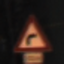
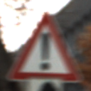
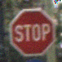
Take a look at these two pictures:
They look almost identical! As a human, you could clearly recognize them as both being stop signs. However one of them really confuses a CNN - despite clearly being a stop sign, the first image (on the left) is being recognized as a “Right of way” sign (meaning “You have the right of way that the next intersection”) - so the exact opposite of what you would want a model to do! In this post, we’ll create the exact images you see right now and show you how to fool a model.
We’ll be using the German Traffic Sign Recognition Benchmark (GTSRB) for this task. The dataset just contains labeled images of german traffic signs, what I want to do is to fool the model to predict a “STOP” sign as a “Right of way” (“Go”) sign.
1. Getting the training data and preprocessing
Before we can start the attack, we need a model of course - in this case, we’re gonna train the model ourselves. It’s going to be a simple, AlexNet inspired model that should be very easy and quick to train (especially since I’m running this notebook locally).
If you don’t really care about this part, feel free to skip to part 4) which contains the actual adversarial attack :)
So far, so good. We now have the dataset on our machine. The next step is to create a pytorch Dataset that manages the image transforms and labels for us.
class TrafficSigns(Dataset):def__init__(self, dataframe, base_path, transforms=v2.Compose([v2.Resize((128, 128)), v2.ToImage(), v2.ToDtype(torch.float32, scale=True)])): data = [ (base_path / x["Path"], x["ClassId"]) for _, x in dataframe.iterrows() ]self.paths, self.labels =list(zip(*data))self.transforms = transformsdef__len__(self):returnlen(self.paths)def__getitem__(self, i): image_path =self.paths[i] label =self.labels[i] image = Image.open(image_path) image =self.transforms(image)return image, torch.tensor(label)train_ds = TrafficSigns(dataframe=pd.read_csv(dataset_path/"Train.csv"), base_path=dataset_path)image, label = train_ds[42]pil_image = v2.ToPILImage()(image)pil_image
Great! We now have a training and validation set which both contain the images! Note the images are loaded “on-demand” (when directly using the dataset). We’re effectively only storing the paths, only if you access an image, the image is opened and loaded.
2) Building the model & training
pickle_path = Path.cwd() /"model.pkl"# Check how many classes there are (assuming all classes are present in the training data)len(set(train_ds.labels))
This will be the architecture we’ll be using. It’s a simple, AlexNet inspired model architecture since it’s easy & efficient to train (I’m actually going to do this on my local machine) and has a relatively high accuracy (although there are of course far better models out there).
from sklearn.metrics import accuracy_score # using accuracy as a metriclearning_rate =1e-4max_lr =2e-3batch_size =64epochs =10loss_fn = torch.nn.CrossEntropyLoss()opt = torch.optim.Adam(model.parameters(), lr=learning_rate)scheduler = torch.optim.lr_scheduler.OneCycleLR(opt, max_lr=max_lr, epochs=epochs, steps_per_epoch=batch_size)train_dl = DataLoader(train_ds, batch_size=batch_size, shuffle=True)valid_dl = DataLoader(valid_ds, batch_size=batch_size)
I’ve adapted some “slight” optimizations such as one-cycle fitting (a LR scheduler) to improve the training speed.
from tqdm import tqdmimport pickledef print_accuracy(epoch, model): model.eval()# Disable gradient calculation for validation accuracywith torch.no_grad(): correct_count =0for x, y in valid_dl: y_pred = model(x).argmax(dim=1) correct_count += (y_pred == y).long().sum().item()print(f"Epoch {epoch} | Accuracy: {correct_count / (batch_size *len(valid_dl))}")if pickle_path.exists():print("Trained model found, skipping training...")withopen(pickle_path, "rb") as pickle_file: model = pickle.load(pickle_file) model, train_dl, valid_dl = accelerator.prepare( model, train_dl, valid_dl )else:print("No trained model found, training instead...") opt = torch.optim.Adam(model.parameters(), lr=learning_rate) model, opt, train_dl, valid_dl, scheduler = accelerator.prepare( model, opt, train_dl, valid_dl, scheduler )for epoch inrange(epochs): model.train()for x, y in tqdm(train_dl): opt.zero_grad() y_pred = model(x) loss = loss_fn(y_pred, y) accelerator.backward(loss) opt.step() scheduler.step() print_accuracy(epoch +1, model)withopen(pickle_path, "wb+") as pickle_file: pickle.dump(model, pickle_file)
Trained model found, skipping training...
3) Quick evaluation
Code
category_labels = ["20km/h","30km/h","50km/h","60km/h","70km/h","80km/h","80km/h aufgehoben","100km/h","120km/h","Überholverbot","Überholverbot (nur LKW)","Vorfahrt an der nächsten Kreuzung","Vorfahrtsstraße","Vorfahrt gewähren","Stop","Einfahrt verboten","Einfahrt verboten (LKW)","Durchfahrt verboten","Gefahr","scharfe Kurve (links)","scharfe Kurve (rechts)","kurvige Strecke","Bodenwellen","Schleudergefahr","verengte Fahrbahn (rechts)","Bauarbeiten","Ampel","Zebrastreifen (Achtung)","spielende Kinder","Fahrradfahrer","Glätte","Wildwechsel","Aufhebung aller Beschränkungen","Nur rechts abbiegen","Nur links abbiegen","Nur geradeaus","Nur geradeaus / rechts","Nur geradeaus / links","Rechts vorbeifahren","Links vorbeifahren","Kreisverkehr","Ende Überholverbot","Ende Überholverbot (LKW)",]# Put the model in evaluation modemodel.eval();
Now that we have all of the labels, we can quickly check our performace.
from sklearn.metrics import classification_report, ConfusionMatrixDisplayimport matplotlib.pyplot as plt# Get predictions for the whole valid datasety_pred = torch.tensor([])y_true = torch.tensor([])for x, y in tqdm(valid_dl): preds = model(x).argmax(dim=1).cpu() y_pred = torch.cat((y_pred, preds)) y_true = torch.cat((y_true, y.cpu()))
from sklearn.metrics import accuracy_scoreprint(f"Classification accuracy: {100* accuracy_score(y_true, y_pred):.2f}%")
Classification accuracy: 95.51%
Not a perfect result, but good enough for our case. We could have of couse optimized further (more epochs, data augmentations, learning rate scheduling, different architecture, …).
4) Creating the adversarial attack
Once we have trained the model, we are finally able to alter an image in such a way that it “tricks” our model. Our model we trained is for sure not the best available one, but it’s a great pick for this notebook since it can be trained very quickly and cheaply.
The goal is to trick the model into recognizing a “STOP” sign as a “right of way sign” by using subtle manipulations that cannot be detected by the human eye.
Now we know how these images look like. Imagine building a self-driving car that uses our approach to recognize these traffic signs. Falsly recognizing a STOP sign as a right-of-way sign could have catastrophic effects and lead to dangerous accidents.
How do we now modify the stop sign in such a way that the model thinks its a ROW (right of way) sign?
Well, the key lies in gradients - we can use them kind of like we use them for training. Remember what a gradient is and how it’s used: Gradients tell us how we have to adapt a set of variables to minimize (or maximize) a function. During training, we use gradients to minimize the loss by adapting the model parameters. Now we want to maximize the loss by changing the image.
Let’s first use the normal loss to try and trick the model into thinking the image is another type of sign, but not necessarily a right of way sign. After we’ve successfully accomplished that, we can move on with the other attack.
model.eval();
We have to make sure the model is in eval-Mode, otherwise the batch norm and dropout layers would mess up our results.
# Turn the image into a 128x128 tensorimg_transforms = v2.Compose( [v2.Resize((128, 128)), v2.ToImage(), v2.ToDtype(torch.float32, scale=True)])
We’re actually all set! We can now pass the image through the model and run the gradient calculation.
img = img.to(accelerator.device)img.retain_grad() # To ensure the gradient is storedpred = model(img[None, :]) # this adds the batch dimension as the model is expecting the image to have dimension [b x c x w x h]pred.argmax(dim=1).item()
Now remember again what the gradient is. The gradient indicates the direction of steepest ascent; if we modify our image in the direction of the gradient, we should maximize the loss and therefore our model should give us another output for the modified image.
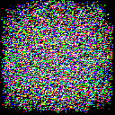
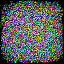
As we can see, a large portion of the gradient seems to be some weird uniform greyish noise - we can’t really see the meaningful parts. Let’s subtract the mean to get a look at the variance of the gradient.
Finally we got a good look at the gradient! It was kind of expectable that the gradient is very small since the STOP sign is probably a very clear example of what the model has stored in its internal representation.
img = img.detach()
Let’s now manipulate the image by gradually adding the gradient until the model makes a wrong prediction.
You might have noticed that I didn’t directly use the gradient here. Instead, I used the sign of the gradient instead. This is reffered to as the Fast Gradient Sign Method to generate adversarial examples, first mentioned by Ian Goodfellow in a paper. You can read more about the original approach here.
After trying around a bit and noising the image; we now got the model to predict something else, in our case the “20km/h” sign with a pretty high confidence (~84.42%)! Now we want to see if we can steer this behavior in some direction.
5) Targetting certain classes
Remember, we take the gradient of the loss functionwith respect to the weights. That means that we calculate the change of the loss function by adapting the weights. Hence, if we want the model to predict a certain other class, we’d just have to adapt our loss function - or alternatively just use the provided loss with a different label. Let’s try the 2nd option first as it’s easier.
category_labels.index("Vorfahrtsstraße")
12
“Vorfahrtsstraße” is the german word for “Right of way sign” - the one we want the model to detect.
img = img_transforms(stop_sign_image)img = img.requires_grad_()img = img.to(accelerator.device)img.retain_grad() # To ensure the gradient is storedpred = model(img[None, :]) # this adds the batch dimension as the model is expecting the image to have dimension [b x c x w x h]loss_fn = torch.nn.CrossEntropyLoss()loss = loss_fn(pred, torch.tensor([12]).to(accelerator.device))loss
There’s not really much to see here, but we can see that the gradient is a bit larger (and with higher magnitude, take a look at the min / max values and compare them to the previous example in section 4) since we would have to change the pixels quite a bit for our image to resemble a right of way sign.
Wow that worked really well! Contrary to the fast sign gradient method, we just did gradient descent on the image here instead to minimize the loss for the right of way sign. In our case, this took just one single try to make the model think the sign was in fact a right of way sign with 89.75% confidence!
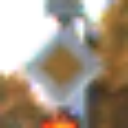
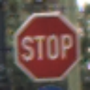
resize(stop_sign_image)
For comparison, here’s the original image.
category_labels[preds.argmax(dim=1).item()]
'Vorfahrtsstraße'
As we can see, we were sucessfull with this very simple approach. There are more sophistiacted approaches out there such as “Projected Gradient Descent” which is very similar to what we did, but ensures that the manipulated image does not exceed a certain perturbation limit (usually also multiple steps are done), see here and here if you want to know more.
With LLMs hitting the mainstream nowadays, studying adversarial attacks on LLMs is also somewhat interesting. If you want to find out more about that, see here.
I hope this post was somewhat interesting, helpful and a somewhat gentle introduction into adversarial attacks, I always appreciate feedback :)